Automatizace ve fyzice: PHYSBO

Petr Čermák

2024-12-05

Připojte se

cermak.science/teaching/automation/lectures/09-physbo/

Opakování

Gaussovský proces

  • neparametrický model náhodného procesu
  • popisuje ho střední hodnota a kovarianční funkce
Ukaž kód
import numpy as np
from helper import plot_gp

def kernel(X1, X2, l=1.0, sigma=1.0):
    """
    Isotropic squared exponential kernel.
    
    Args:
        X1,2: Array of m points (m x d).
        X2: Array of n points (n x d).

    Returns:
        (m x n) matrix.
    """
    sqdist = np.sum(X1**2, 1).reshape(-1, 1) + np.sum(X2**2, 1) - 2 * np.dot(X1, X2.T)
    return sigma**2 * np.exp(-0.5 / l**2 * sqdist)


# Vygeneruji body (konečný počet)
X = np.arange(0, 10, 0.1).reshape(-1, 1) #počet sloupců dopočítá

mu = np.zeros(X.shape)   # střední hodnota
cov = kernel(X, X)       # spočtu kovarianci (nenormovaná korelace)

# Vygeneruji 5 funkcí jako výsledek náhodného gaussovského procesu
samples = np.random.multivariate_normal(mu.ravel(), cov, 5)

# Vykreslí střední hodnotu, oblast nejistoty a funkce 
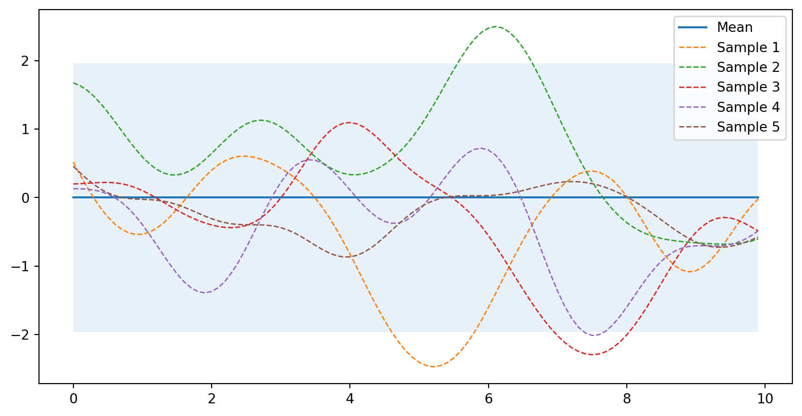
plot_gp(mu, cov, X, samples=samples)

Posterior

Ukaž kód
from numpy.linalg import inv

def posterior(X, X_train, Y_train, l=1.0, sigma=1.0, sigma_y=1e-8):
    """
    Spočítá novou střední hodnotu a kovarianci při znalosti train dat
    
    Args:
        X: osa x
        X_train, Y_train: známá data (m x 1)
        l, sigma: Parametry jádra
        sigma_y: šum
    
    Returns:
        Posterior střední hodnota (n x d) a kovariance (n x n).
    """
    K = kernel(X_train, X_train, l, sigma) + sigma_y**2 * np.eye(len(X_train))  # jádro s šumem
    K_s = kernel(X_train, X, l, sigma)
    K_ss = kernel(X, X, l, sigma) + 1e-8 * np.eye(len(X))
    
    # Equation (7)
    mu_s = K_s.T.dot(inv(K)).dot(Y_train)
    # Equation (8)
    cov_s = K_ss - K_s.T.dot(inv(K)).dot(K_s)
    return mu_s, cov_s


noise = 0.2
X_train = np.arange(0, 5, 1).reshape(-1, 1)
Y_train = np.sin(X_train) + noise * np.random.randn(*X_train.shape)
mu_s, cov_s = posterior(X, X_train, Y_train, sigma_y=noise)
samples = np.random.multivariate_normal(mu_s.ravel(), cov_s, 3)
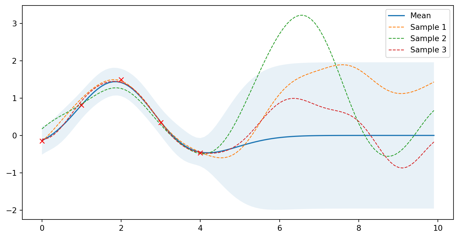
plot_gp(mu_s, cov_s, X, X_train=X_train, Y_train=Y_train, samples=samples)

\[ \kappa(\mathbf{x}_i,\mathbf{x}_j) = \sigma^2 \exp\left(-\frac{\|\mathbf{x}_i - \mathbf{x}_j\|^2}{2l^2}\right) \]

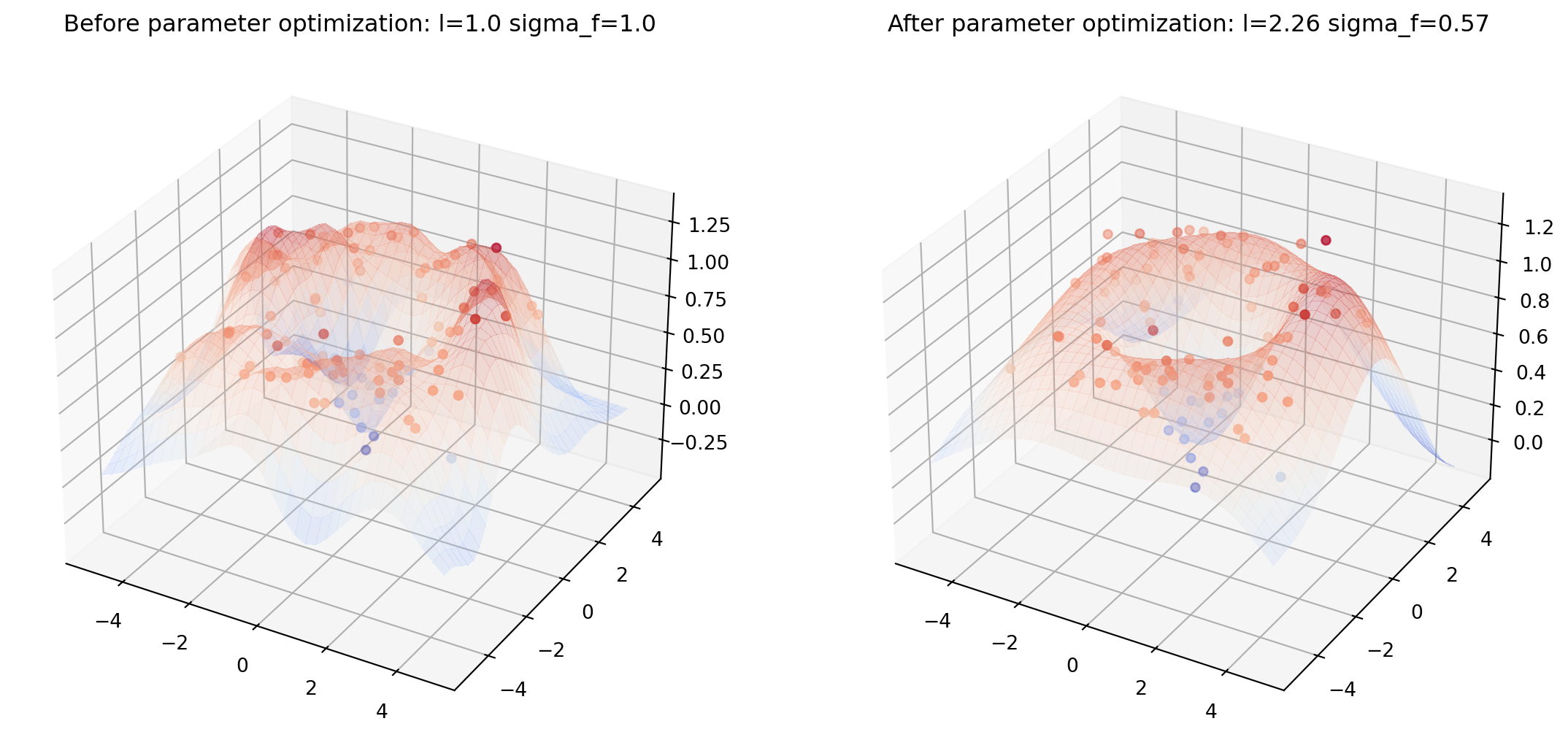
Optimální parametry se musí fitovat

Kód zde
from numpy.linalg import cholesky, det
from scipy.linalg import solve_triangular
from scipy.optimize import minimize
from matplotlib import pyplot as plt

def nll_fn(X_train, Y_train, noise, naive=True):
    """
    Returns a function that computes the negative log marginal
    likelihood for training data X_train and Y_train and given
    noise level.

    Args:
        X_train: training locations (m x d).
        Y_train: training targets (m x 1).
        noise: known noise level of Y_train.
        naive: if True use a naive implementation of Eq. (11), if
               False use a numerically more stable implementation.

    Returns:
        Minimization objective.
    """
    
    Y_train = Y_train.ravel()
    
    def nll_naive(theta):
        # Naive implementation of Eq. (11). Works well for the examples 
        # in this article but is numerically less stable compared to 
        # the implementation in nll_stable below.
        K = kernel(X_train, X_train, l=theta[0], sigma=theta[1]) + \
            noise**2 * np.eye(len(X_train))
        return 0.5 * np.log(det(K)) + \
               0.5 * Y_train.dot(inv(K).dot(Y_train)) + \
               0.5 * len(X_train) * np.log(2*np.pi)
        
    def nll_stable(theta):
        # Numerically more stable implementation of Eq. (11) as described
        # in http://www.gaussianprocess.org/gpml/chapters/RW2.pdf, Section
        # 2.2, Algorithm 2.1.
        
        K = kernel(X_train, X_train, l=theta[0], sigma=theta[1]) + \
            noise**2 * np.eye(len(X_train))
        L = cholesky(K)
        
        S1 = solve_triangular(L, Y_train, lower=True)
        S2 = solve_triangular(L.T, S1, lower=False)
        
        return np.sum(np.log(np.diagonal(L))) + \
               0.5 * Y_train.dot(S2) + \
               0.5 * len(X_train) * np.log(2*np.pi)

    if naive:
        return nll_naive
    else:
        return nll_stable


from helper import plot_gp_2D

noise_2D = 0.1

rx, ry = np.arange(-5, 5, 0.3), np.arange(-5, 5, 0.3)
gx, gy = np.meshgrid(rx, rx)

X_2D = np.c_[gx.ravel(), gy.ravel()]

X_2D_train = np.random.uniform(-4, 4, (100, 2))
Y_2D_train = np.sin(0.5 * np.linalg.norm(X_2D_train, axis=1)) + \
             noise_2D * np.random.randn(len(X_2D_train))

plt.figure(figsize=(14,7))

mu_s, _ = posterior(X_2D, X_2D_train, Y_2D_train, sigma_y=noise_2D)
plot_gp_2D(gx, gy, mu_s, X_2D_train, Y_2D_train, 
           f'Before parameter optimization: l={1.00} sigma_f={1.00}', 1)

res = minimize(nll_fn(X_2D_train, Y_2D_train, noise_2D), [1, 1], 
               bounds=((1e-5, None), (1e-5, None)),
               method='L-BFGS-B')

mu_s, _ = posterior(X_2D, X_2D_train, Y_2D_train, *res.x, sigma_y=noise_2D)
plot_gp_2D(gx, gy, mu_s, X_2D_train, Y_2D_train,
           f'After parameter optimization: l={res.x[0]:.2f} sigma_f={res.x[1]:.2f}', 2)
Bayesovská optimalizace

Cíl: najít minimum za pomocí nejmenšího počtu měření

–> Bayesovská optimalizace! Potřebujeme:

Surrogate model

  • Gaussovský proces

Akviziční funkce

  • hledá kompromis mezi
    • průzkumem (exploration) - měřit tam, kde nic nevíme
    • vytěžováním (exploitation) - měřit tom, kde se odhaduje minimum/maximum

Optimalizační tooly

PHYSBO

optimization tools for PHYsics based on Bayesian Optimization

  • práce s mnohem většími daty než scikit-learn
  • snadné a uživatelsky přívětivé
  • mnoho tutoriálů

Základní syntaxe

import itertools, physbo, numpy as np
from random import random

#muj rozsah promennych
xrange = np.linspace(-1,1,41)
yrange = np.linspace(-1,1,41)
X = np.array(list(itertools.product(xrange, yrange)))

#moje měřící funkce
class Cooking:
  def __init__(self):
    self._secret_x = random() * 2 - 1
    self._secret_y = random() * 2 - 1
    print(f"secret position is {self._secret_x},{self._secret_y}")

  def __call__(self, actions):
    action_idx = actions[0]
    x = X[action_idx][0]
    y = X[action_idx][1]
    return -(x - self._secret_x)**2 - (y - self._secret_y)**2 + 1   

mycooking = Cooking()
# nastavit seed a oblast hledani
policy = physbo.search.discrete.policy(test_X=X)
policy.set_seed(0)
#nahodne hledani (min. 2 vzorky)
res = policy.random_search(max_num_probes=10, simulator=mycooking)
#Bayesovske hledani
res = policy.bayes_search(max_num_probes=20, simulator=mycooking, 
                          score='TS', interval=0, num_rand_basis=500)
bestid = policy.history.export_sequence_best_fx()[1][-1]
print(f"Reached best value for sample #{bestid} with {X[bestid]}")

Základní syntaxe

secret position is -0.5009378811598519,-0.054392957797946284
0001-th step: f(x) = -0.060423 (action=1018)
   current best f(x) = -0.060423 (best action=1018) 

0002-th step: f(x) = 0.594333 (action=605)
   current best f(x) = 0.594333 (best action=605) 

0003-th step: f(x) = 0.935787 (action=596)
   current best f(x) = 0.935787 (best action=596) 

0004-th step: f(x) = 0.727860 (action=836)
   current best f(x) = 0.935787 (best action=596) 

0005-th step: f(x) = 0.247230 (action=569)
   current best f(x) = 0.935787 (best action=596) 

0006-th step: f(x) = -0.068865 (action=857)
   current best f(x) = 0.935787 (best action=596) 

0007-th step: f(x) = 0.974259 (action=553)
   current best f(x) = 0.974259 (best action=553) 

0008-th step: f(x) = 0.499545 (action=1001)
   current best f(x) = 0.974259 (best action=553) 

0009-th step: f(x) = -0.210956 (action=1060)
   current best f(x) = 0.974259 (best action=553) 

0010-th step: f(x) = 0.622470 (action=540)
   current best f(x) = 0.974259 (best action=553) 

Start the initial hyper parameter searching ...
Done

Start the hyper parameter learning ...
0 -th epoch marginal likelihood -3.8973554824877876
50 -th epoch marginal likelihood -4.270263628042907
100 -th epoch marginal likelihood -4.582284029440011
150 -th epoch marginal likelihood -4.849787786564914
200 -th epoch marginal likelihood -5.08474579027653
250 -th epoch marginal likelihood -5.294954048477102
300 -th epoch marginal likelihood -5.4857195241763295
350 -th epoch marginal likelihood -5.660797090993938
400 -th epoch marginal likelihood -5.822928451072767
450 -th epoch marginal likelihood -5.9741682854682505
500 -th epoch marginal likelihood -6.116090237213503
Done

0011-th step: f(x) = 0.978914 (action=513)
   current best f(x) = 0.978914 (best action=513) 

0012-th step: f(x) = -1.336424 (action=1394)
   current best f(x) = 0.978914 (best action=513) 

0013-th step: f(x) = -0.143236 (action=0)
   current best f(x) = 0.978914 (best action=513) 

0014-th step: f(x) = 0.995325 (action=469)
   current best f(x) = 0.995325 (best action=469) 

0015-th step: f(x) = 0.986853 (action=512)
   current best f(x) = 0.995325 (best action=469) 

0016-th step: f(x) = 0.977198 (action=552)
   current best f(x) = 0.995325 (best action=469) 

0017-th step: f(x) = 0.989792 (action=511)
   current best f(x) = 0.995325 (best action=469) 

0018-th step: f(x) = 0.986507 (action=472)
   current best f(x) = 0.995325 (best action=469) 

0019-th step: f(x) = 0.948410 (action=351)
   current best f(x) = 0.995325 (best action=469) 

0020-th step: f(x) = 0.994447 (action=471)
   current best f(x) = 0.995325 (best action=469) 

0021-th step: f(x) = 0.997386 (action=470)
   current best f(x) = 0.997386 (best action=470) 

0022-th step: f(x) = 0.966320 (action=554)
   current best f(x) = 0.997386 (best action=470) 

0023-th step: f(x) = 0.997041 (action=430)
   current best f(x) = 0.997386 (best action=470) 

0024-th step: f(x) = 0.987732 (action=510)
   current best f(x) = 0.997386 (best action=470) 

0025-th step: f(x) = 0.999980 (action=429)
   current best f(x) = 0.999980 (best action=429) 

0026-th step: f(x) = 0.989101 (action=431)
   current best f(x) = 0.999980 (best action=429) 

0027-th step: f(x) = 0.994634 (action=389)
   current best f(x) = 0.999980 (best action=429) 

0028-th step: f(x) = 0.973568 (action=473)
   current best f(x) = 0.999980 (best action=429) 

0029-th step: f(x) = 0.975138 (action=551)
   current best f(x) = 0.999980 (best action=429) 

0030-th step: f(x) = 0.986695 (action=390)
   current best f(x) = 0.999980 (best action=429) 

Reached best value for sample #429 with [-0.5  -0.05]

Přehled akvizičních funkcí

Probability of Improvement (PI)

  • Maximalizuje pravděpodobnost, že nové vyhodnocení přinese zlepšení oproti dosavadnímu maximu.
  • Rychlé a jednoduché.
  • Může opomenout průzkum, vhodné u optima.

Expected Improvement (EI)

  • Maximalizuje očekávanou hodnotu zlepšení oproti dosavadnímu maximu.
  • Vyvážený exploration vs. exploitation.
  • Výpočetně náročnější než PI.

Thompson Sampling (TS)

  • Náhodně vzorkuje z posterioru predikovaného modelu a vybírá body s vysokou pravděpodobností optima.
  • Efektivní průzkumný přístup, vhodný pro paralelní evaluace.
  • Může vést k příliš velkému průzkumu v některých případech.

Průzkum: Thompson Sampling

Vyhledávání: PI, EI

Univerzální scénáře: EI

Výpočetně omezené scénáře: PI

Úkol #3

Zadání

  • Existuje lanýžový les o rozloze 100x100m
  • Každý má k dispozici jedno virtuální prase
  • Kopání:
    • je třeba určit praseti kde kopat (x,y)
    • prase zjistí, kolik lanýžů je pod zemí (max 255)
  • Prase musí po kopání 5 minut odpočívat
  • Cíl: najít oblast s nejvyšší množstvím lanýžů
  • Cíl 2: prase každým kopáním stárne, chceme najít maximum a přitom prase co nejméně obtěžovat

Jak na to?

  • získat vstupenku do lesa: napíšeme robotovi: $get_forest_permit

https://user.mgml.eu/forest/?x=XX&y=YY&permit=abcdef

  • vrátí to chybu (HTTP 500) nebo ok (code 200)